Excel で乗算する 3 つの方法(アスタリスクと関数を使用)

D3 セルと E3 セルを掛けます。選ぶ[Cell (F3 cell in example)]をクリックして乗算結果を表示し、「=D3」と入力します。等しいと入力した後に「D3」と入力する代わりに、D3 セルを選択しても同様です。

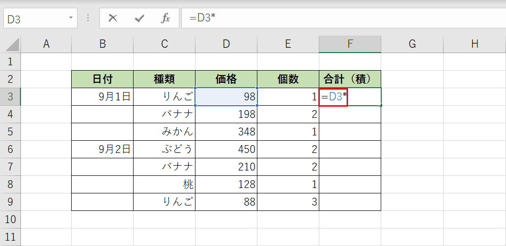
=D3 の後に *(アスタリスク) と入力します。

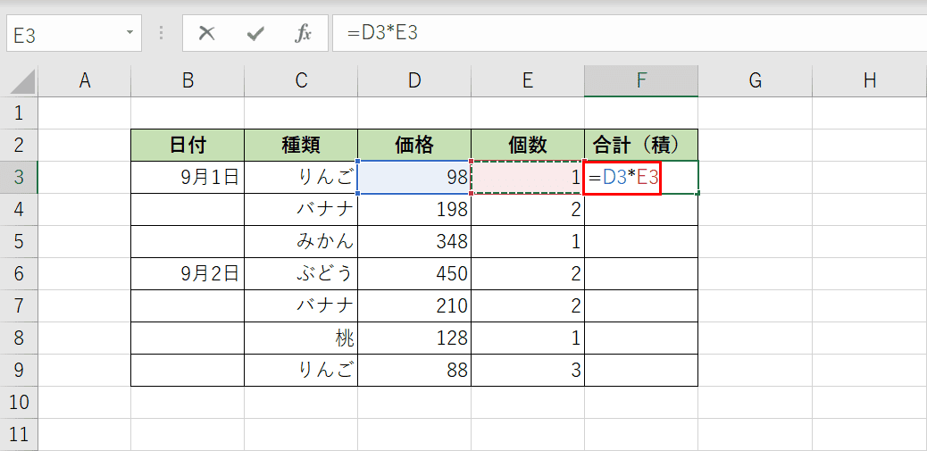
タイプ =D3* の後に E3 を入力します。入力する代わりに E3 セルを選択しても同じことが言えます。

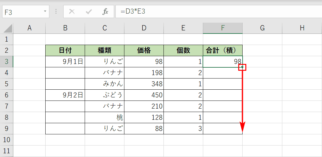
F3セルにD3セルとE3セルを掛けた結果を「98」と表示し、F3セルの右下をF9セルにドラッグする。

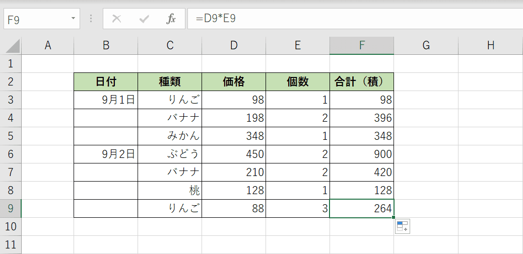
列 D と列 E の乗算の結果が列 F に表示されました。"*" (アスタリスク) を使用すると簡単に乗算できます。

D3 セルと E3 セルを掛けます。選ぶ[Cell (in example, F3 cell)]乗算結果を表示する場所に、"=PRODUCT(" と関数名を入力します。

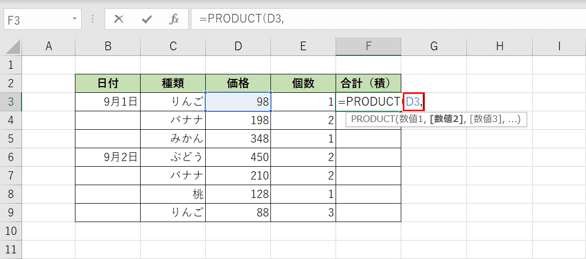
“=PRODUCT(" の後に “D3,"" と入力するか、D3 セルを選択します。

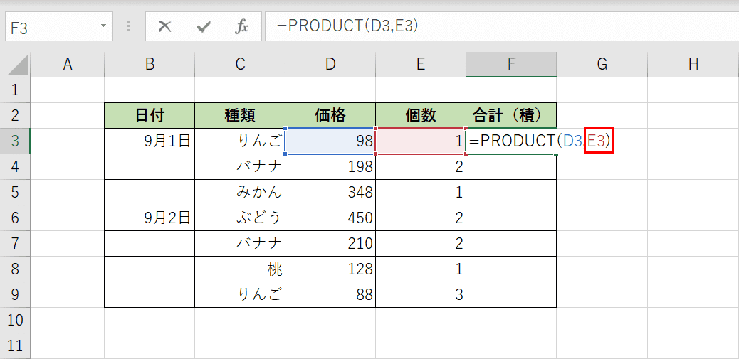
タイプ =プロダクト(D3,,"]E3が続きます。または、E3 セルを選択します。最後です入る押す。

PRODUCT関数を用いてF3セルにD3セルとE3セルを掛けた結果、「98」と表示されました。

D3 セルと E3 セルを掛けます。選ぶ[Cell (F3 cell in example)]をクリックして乗算結果を表示し、関数名に “=SUMPRODUCT(" と入力します。

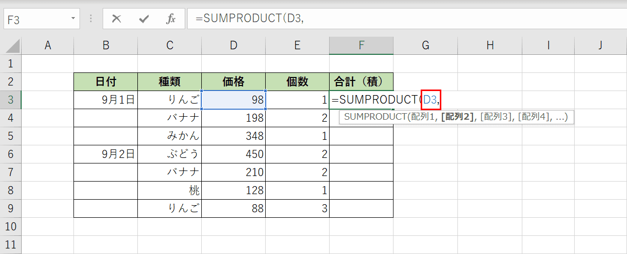
「=SUMPRODUCT(」の後に D3″ と入力するか、D3 セルを選択します。

=SUMPRODUCT(D3,,"]と入力してください。

E3が続きます。または、E3 セルを選択します。最後です入る押す。

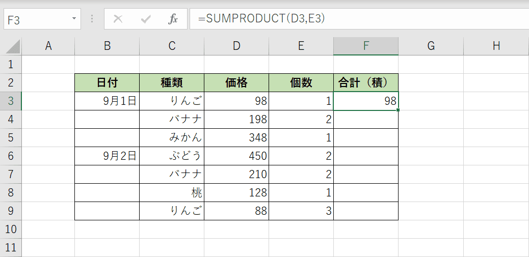
SUMPRODUCT関数を用いてF3セルにD3セルとE3セルを掛けた結果、「98」と表示されました。

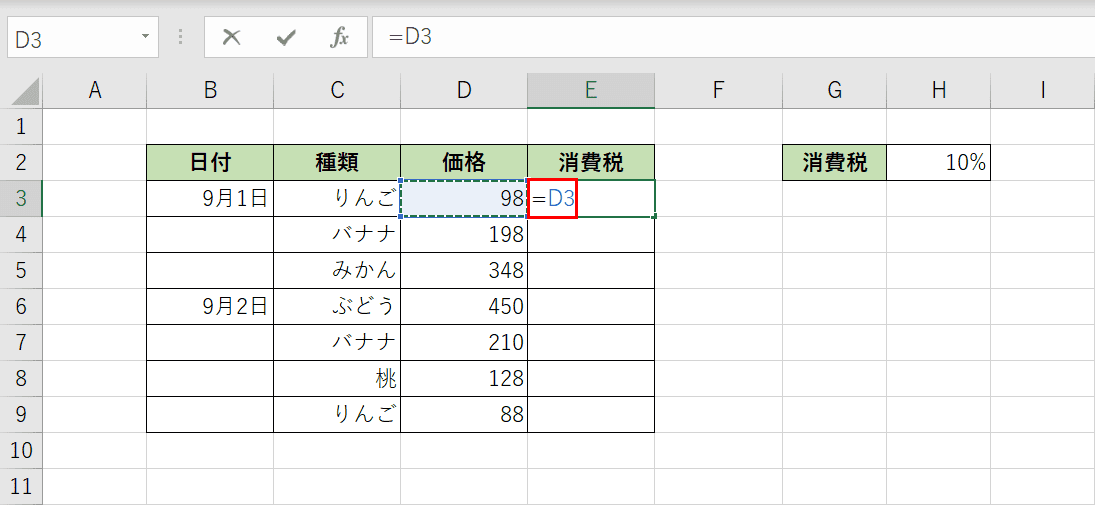
D3 セルと H2 セルを掛けます。選ぶ[Cell(E3cellineg)whereyouwanttodisplaythemultipliedresultandenter"=D3″

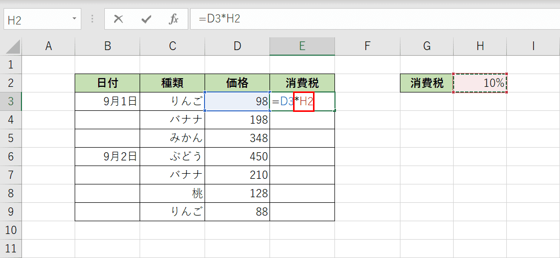
Type =D3 followed by *H2. If you display the result as it is, the correct result will be displayed in the E3 cell, but the H2 cell will be misalized when copying with autofill.

Let’s make the H2 cell an absolute reference.

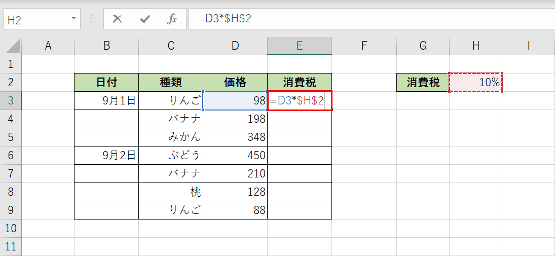
F4to change H2 to $H$2.Enterto confirm.

The D3 and H2 cell multiplication results were displayed as “9.8" in the E3 cell. Drag the lower right of the E3 cell to the E9 cell to autofill.

The result of fixing the H2 cell with an absolute reference and multiplying it by column D could be displayed in column E.

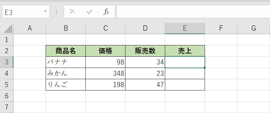
It is a method of multiplication together by column. It is a method of calculating the sales of bananas, mandarin oranges, and apples at once.

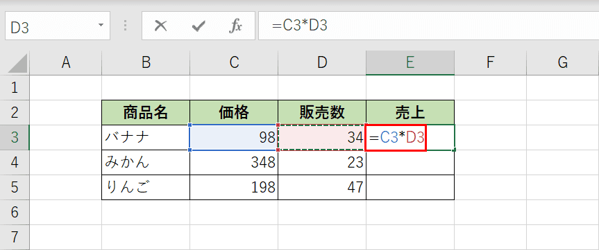
First, select the E3 cell and enter =C3*D3.

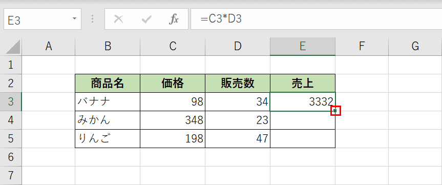
The sales were calculated as 3332, and the square of the red frame at the bottom right of the cell is called the fill handle. Let’s[double click]これ。

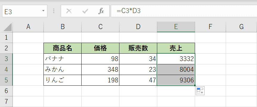
その後、E4およびE5セルが自動的に計算された。横の列と縦の列の計算にも同じことができるので、試してみましょう。

列 D の価格の合計に列 E の数を掛けた値を F10 セルで表示します。

F10 セルを選択し、セルに直接 =SUMPRODUCT() と入力します。

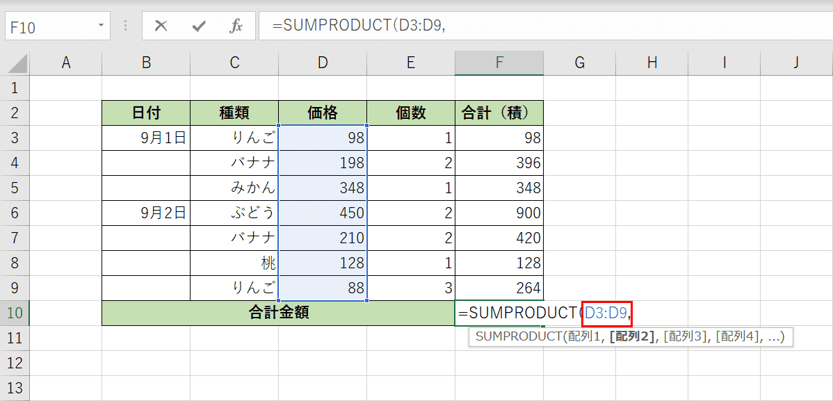
D3 から D9 のセル範囲にドラッグして選択するか、=SUMPRODUCT と入力します (その後に D3:D9," と入力します)。

範囲を E3 から E9 セルにドラッグして選択するか、=SUMPRODUCT (D3:D9,,") と入力して E3:E9 と入力します。最後に、式入る押す。

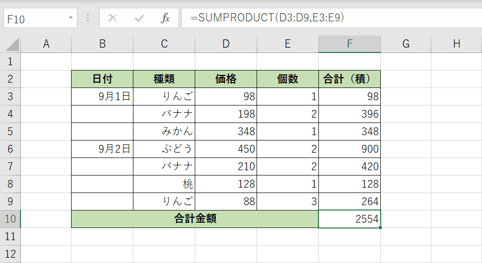
F10セルのSUMPRODUCT関数を使用して乗算した結果の合計を表示することができました。